To understand , a term used to describe a very quick push or pull on a system, such as the blow of a hammer or the force of an explosion, and that an impulse function can be described by , \(\delta(t)\text<,>\) which has the properties
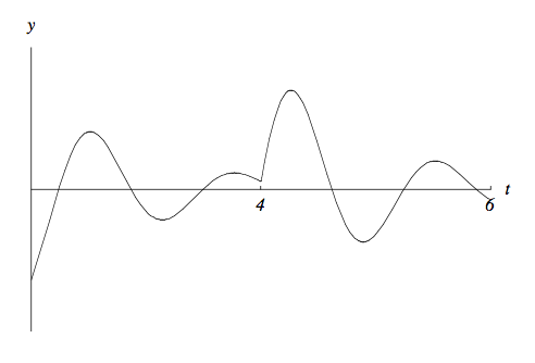
\begin \delta(t) = 0, \qquad t \neq 0;\\ \int_<-\infty>^ <\infty>\delta(t) \, dt = 1. \end To understand that we can use the Dirac delta function to solve initial value problems such as \begin \frac + 2 \frac + 26 y & = \delta_4(t)\\ y(0) & = 1\\ y'(0) & = 0, \end \begin \frac + p \frac + q y = g(t), \end where \(g(t)\) is a function that is very large in a very short time interval.is the term used to describe a very quick push or pull on a system, such as the blow of a hammer or the force of an explosion. For example, consider the equation for a damped harmonic oscillator
\begin \frac + 2 \frac + 26 y = g(t), \endwhere \(g(t)\) is a function that is very large in a very short time interval, say \(|t - t_0| \lt \tau\) and zero otherwise. The integral
\begin I(\tau) = \int_^ g(t) \, dt \end or since \(g(t)\) is zero outside of the interval \(|t - t_0| \lt \tau\) \begin I(\tau) = \int_<-\infty>^ <\infty>g(t) \, dt \endmeasures the strength or of the forcing function \(g(t)\text<.>\) In particular, assume that \(t_0 = 0\) and
\begin g(t) = d_(t) = \begin 1/ 2\tau, & -\tau \lt t \lt \tau \\ 0, & \text \end \end It is easy to see that \(I(\tau) = 1\) in this case.Examining this forcing function over shorter and shorter time intervals with \(\tau\) getting closer and closer to zero, we find that \(I(\tau) = 1\) in all cases. Thus,
\begin \lim_ d_\tau(t) = 0 \end for \(t \neq 0\text<;>\) however, \begin \lim_ I(\tau ) = 1. \endWe can use this information to define the , \(\delta(t)\text<,>\) to be the ``function’’ that imparts an impulse of magnitude one at \(t = 0\text<,>\) but is zero for all values of \(t\) other than zero. In other words, \(\delta(t)\) has the properties
\begin \delta(t) = 0, \qquad t \neq 0;\\ \int_<-\infty>^ <\infty>\delta(t) \, dt = 1. \endOf course, we study no such function in calculus. The ``function’’ \(\delta\) is an example of what is known as a . We call \(\delta\text<,>\) the .
We can define a unit impulse at a point \(t_0\) by considering the function \(\delta( t - t_0)\text<.>\) In this case,
\begin \delta(t - t_0) = 0, \qquad t \neq t_0;\\ \int_<-\infty>^ <\infty>\delta(t - t_0) \, dt = 1. \endEven though the Dirac delta function is not a piecewise continuous, exponentially bounded function, we can define its Laplace transform as the limit of the Laplace transform of \(d_\tau(t)\) as \(\tau \to 0\text<.>\) More specifically, assume that \(t_0 \gt 0\) and
\begin <\mathcal L>(\delta(t - t_0)) = \lim_ <\mathcal L>(d_\tau(t - t_0)). \end Assuming that \(t_0 - \tau \gt 0\text<,>\) the Laplace transform of \(d_\tau(t - t_0)\) is We can use l’Hospital’s rule to evaluate \((\sinh s \tau)/ s \tau\) as \(\tau \to 0\text<,>\) \begin \lim_ \frac = \lim_ \frac = 1. \end \begin <\mathcal L>(\delta(t - t_0)) = e^. \end We can extend this result to allow \(t_0 = 0\text<,>\) by \begin \lim_ <\mathcal L>(\delta(t - t_0)) =\lim_ e^ = 1. \endWe can think of this as a damped harmonic oscillator that is struck by a hammer at time \(t = 4\text<.>\) Let \(Y(s) = <\mathcal L>(y)(s)\) and take the Laplace transform of both sides of the differential equation to obtain
\begin s^2 Y(s) - sy(0) - y'(0) + 2(sY(s) - y(0)) + 26 Y(s) = <\mathcal L>(\delta_4)(s) \end \begin s^2 Y(s) - s + 2sY(s) - 2 + 26 Y(s) = e^. \end Solving for \(Y(s)\text<,>\) we have \begin Y(s) = \frac + \frac>. \end The inverse Laplace transform of \(Y(s)\) is
We take the Laplace transformation of both sides. To take the Laplace transformation of \(u_1(t)(t + 1 + \delta_1(t))\text<,>\) we rewrite the factor being multiplied by \(u_1(t)\) replacing \(t\) with \(t+1\text<,>\) giving \(t+2 + \delta_1(t+1) = t + 2 + \delta_0(t+1-1) = t + 2 + \delta_0(t)\text\) take the Laplace of this and multiply by \(e^\text<,>\) giving \(e^(\frac + \frac + 1)\text<.>\) We arrive at the equation
\begin sY(s) + Y(s) = \frac + \frac + e^(\frac + \frac + 1) \end \begin Y(s) = \frac + \frac + e^(\frac + \frac + \frac) \end It looks like we have to do extensive partial fractions, but we don’t; observe that \begin \frac + \frac = \frac = \frac \end and \(\frac<1> + \frac + \frac<1> = \frac = \frac=\frac1s + \frac<1>\) So we end up at the equation \begin Y(s) = \frac + e^(\frac1s + \frac) \endWe now have to take the inverse Laplace to solve for \(y(t)\text<.>\) The first term on the right gives us \(t^2\text<.>\) The inverse Laplace of \(\frac1s + \frac\) is \(1 + t\text<.>\) Since \(\frac1s + \frac\) is multiplied by \(e^\text\) we subtract 1 to the arguments and multiply by \(\delta_1(t)\) to get the inverse Laplace. The final answer is
\begin y(t) = t^2 + \delta_0(t)\cdot t \endIt is important to notice that we are using the Dirac delta function like an ordinary function. This requires some rigorous mathematics to justify that we can actually do this.
is the term used to describe a very quick push or pull on a system, such as the blow of a hammer or the force of an explosion. For example, consider the equation for a damped harmonic oscillator
\begin \frac + p \frac + q y = g(t), \endwhere \(g(t)\) is a function that is very large in a very short time interval, say \(|t - t_0| \lt \tau\) and zero otherwise. The integral
\begin I(\tau) = \int_^ g(t) \, dt \end or since \(g(t)\) is zero outside of the interval \(|t - t_0| \lt \tau\) \begin I(\tau) = \int_<-\infty>^ <\infty>g(t) \, dt \end measures the strength or of the forcing function \(g(t)\text<.>\)We define the , \(\delta(t)\text<,>\) to be the ``function’’ that imparts an impulse of magnitude one at \(t = 0\text<,>\) but is zero for all values of \(t\) other than zero. In other words, \(\delta(t)\) has the properties
\begin \delta(t) = 0, \qquad t \neq 0;\\ \int_<-\infty>^ <\infty>\delta(t) \, dt = 1. \end The “function” \(\delta\) is an example of what is known as a . We call \(\delta\text<,>\) the .Similarly, we can define a unit impulse at a point \(t_0\) by considering the function \(\delta( t - t_0)\text<.>\) In this case,
\begin \delta(t - t_0) = 0, \qquad t \neq 0;\\ \int_<-\infty>^ <\infty>\delta(t - t_0) \, dt = 1. \end The Laplace transform of the Dirac delta function is \begin <\mathcal L>(\delta(t - t_0)) = e^. \end We can extend this result to allow \(t_0 = 0\text<,>\) by \begin \lim_ <\mathcal L>(\delta(t - t_0)) =\lim_ e^ = 1. \end We can use the Dirac delta function to solve initial value problems such as \begin \frac + 2 \frac + 26 y & = \delta_4(t)\\ y(0) & = 1\\ y'(0) & = 0, \end \begin \frac + p \frac + q y = g(t), \end where \(g(t)\) is a function that is very large in a very short time interval.Solve the initial problems in Exercise Group 3.3.5.1–6 using the Laplace transform, \(\delta(t)\) is the unit impulse function.